


Oprah Winfrey coined the phrase: “the ah-ha moment.” She was referring to that exact moment when your brain tells you that you have just learned something new; something important.
Today we will review a podcast that features Steve Hanke, Professor of Applied Economics at The Johns Hopkins University in Baltimore. Here is a link to the podcast and another one to the biography of Professor Hanke:
https://www.cato.org/people/steve-h-hanke
The subject of the podcast was a simple question:
“Why did the FED change its reporting of the Money Supply data?”
This data had previously been published since the 1970s and was being used by economists and investors alike to try to get a better understanding of how the money supply impacts nominal GDP, which includes real growth and inflation.
The Professor takes us back to the 1970s and early 1980s when Paul Volker was the FED Chairman (1979 – 1987). Volker relied on the FED data, particularly the data that related to Money Supply, in his effort to try to curb inflation which was over 10%. The term “stagflation” conveyed a stagnant economy coupled with high inflation.
This was a “government nightmare scenario.” Strong action was required, and Volker took it.
Volker carefully monitored the weekly reporting of M2 and used that data to inform his decision to continue to raise interest rates, which continued to climb to over 20% before they began to fall.
The FED’s implementation of this severe monetary policy also resulted in two recessions, a mild one in 1980 and a more severe one in 1982. Inflation was brought under control but at a cost. Real GDP was also negatively impacted.
Volker slowed down the growth in Money Supply.
Professor Hanke contends that Volker actually created a situation where money supply growth became negative because he was incorrect in his measurement of it.
M1 and M2 are considered to be simple sum indices.
This means they are derived by adding up various constituent inputs. For example, M2 is made up of 9 components, including M1 plus savings deposits, money market funds, certificates of deposit, and other time deposits.
Professor Hanke refers us to another method of looking at M2. The Center for Financial Stability has come up with a different way to assess the components that make up M2. Broadly speaking, it is called the Divisia Index.
The Divisia Index assigns a different degree of “moneyness” to the M2 components. Obviously, currency gets a 100% weighting, as do checking accounts. Both of them can be used immediately for transactions.
The other components of M2 receive less than a 100% weight; however, the weighting shifts around depending on interest rates. For example, during Volker’s tenure as FED Chairman, interest rates soared to double digits. This meant that there was an opportunity cost to exchange your savings account or money market account for cash. It is intuitive to conclude that there would be a natural reluctance to turn savings into cash at a high-interest rate.
So, by using this method to calculate M2, it went negative in the early 1980s. Volcker, not having access to this data, thought that he had gotten M2 growth down to around 7%, when in fact, it was much lower. This negative growth in M2 resulted in the two recessions in the early 1980s.
By contrast, the current FED Chairman has been very clear in expressing his belief that M2 is unrelated to inflation.
The FED has changed its reporting of M2 from weekly to monthly. This was done in an effort to shift attention away from money supply growth.
So, let’s take a step back in time and review the last time the FED made a significant change to the reporting of the money supply.
Do you remember this announcement by the FED?
Discontinuance of M3
“On March 23, 2006, the Board of Governors of the Federal Reserve System will cease publication of the M3 monetary aggregate. The Board will also cease publishing the following components: large-denomination time deposits, repurchase agreements (RPs), and Eurodollars. The Board will continue to publish institutional money market mutual funds as a memorandum item in this release.
Measures of large-denomination time deposits will continue to be published by the Board in the Flow of Funds Accounts (Z.1 release) on a quarterly basis and in the H.8 release on a weekly basis (for commercial banks).
M3 does not appear to convey any additional information about economic activity that is not already embodied in M2 and has not played a role in the monetary policy process for many years. Consequently, the Board judged that the costs of collecting the underlying data and publishing M3 outweigh the benefits.”
The FED stopped their reporting of M3 in 2006. Do you remember what happened just a few short years later?
Right. The Financial Crisis of 2008.
Some people contend that by no longer providing M3 data, the FED obscured the interpretation of what was happening in the massively overleveraged derivative market.
Short-term debt instruments created out of the slicing up of risky and faulty mortgage-backed securities were hidden from view. It was as though the FED deliberately made it more difficult to observe and react to the lurking debt iceberg created by the invention of mortgage-backed debt securities and their related financial instruments.
When credit markets “froze” in 2008 and banks no longer trusted each other when it came to “overnight” lending, the entire global financial system was threatened.
The solution?
Massive bailouts of large banks – the FED created more money which was used to improve the balance sheets and corresponding reserve ratios of large banks so that they would not be in default.
There is a singular focus on 2008, but perhaps it is more reasonable to consider the actions of the FED in 2006 as a precursor to their subsequent requisite action (QE) in 2008.
Now, not to be an alarmist, but isn’t it a bit strange to see the FED, once again, take a position of less disclosure when it comes to reporting various elements that comprise the money supply?
Will we need another “2 years” to find out why the FED adopted these new money supply reporting protocols?
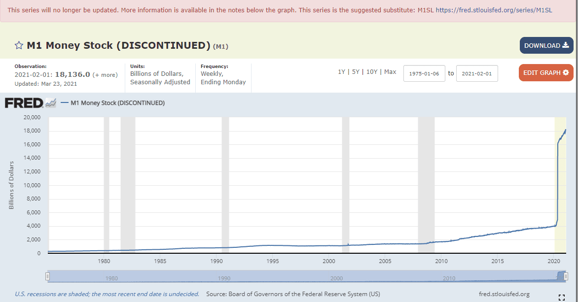
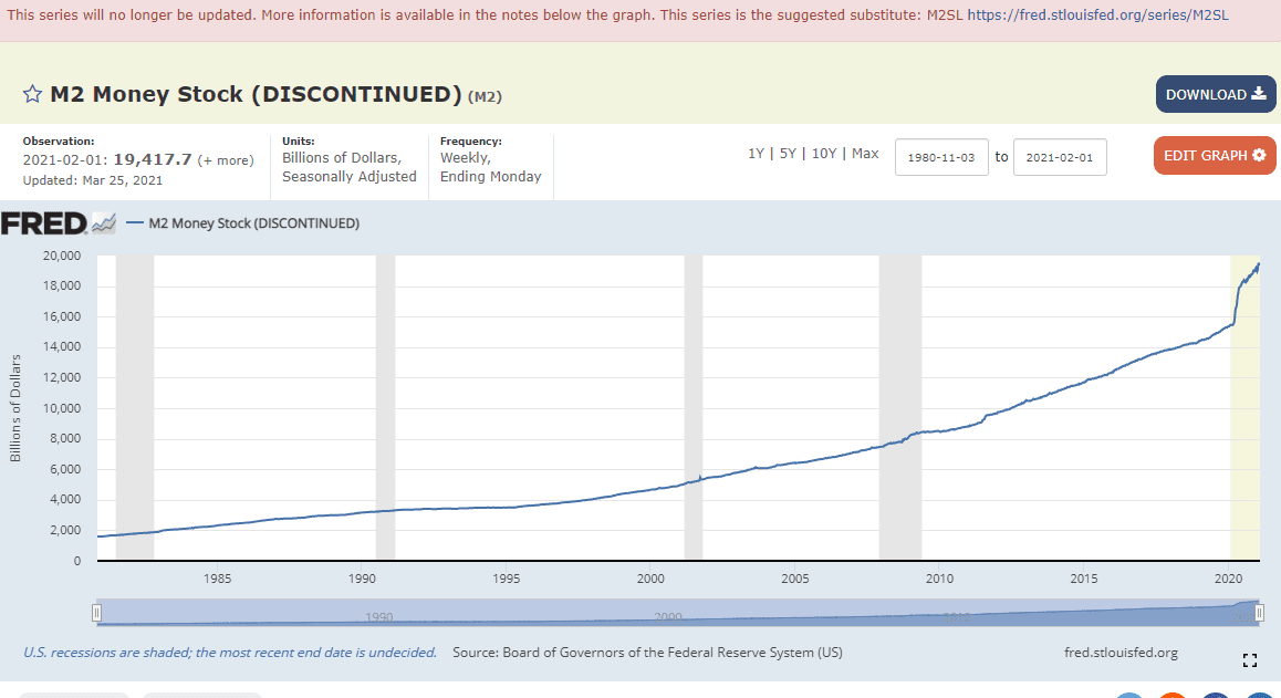
Here is a last look at the weekly chart showing the M2 and M1 money supply graphs, which will now report only monthly.
The FED wants to control inflation expectations.
How can this be achieved? One way is to reduce the annual views of these two graphs from 52 times per year to 12.
When they look at these graphs, most people conclude that inflation will be a natural outcome of the massive money supply growth that has taken place. They are not wrong.
Professor Hanke walks us through an example of what happens when monetary policy is tightened. This is achieved by raising short-term interest rates. Money supply drops, leading to a drop in nominal GDP and inflation drops. Sustained longer-term interest rates then drop. This action leads to a confusing economic signal. The opposite occurs during a period when monetary policy is loosened, as it is today. Money supply growth has exploded, as the graphs clearly indicate.
This explanation of how money supply growth ties into interest rates by Professor Hanke also makes it easy to understand why the bond market has “sprung to life” in recent months.
CPI is rising by 1.7% per annum, the PPI (producer price index) is rising by 2.8%, and a measure of food prices shows an annual increase of 3.6%.
There are numerous “inflation baskets” – the FED has mandated inflation targeting as a key policy goal. But what exactly is inflation? What components are they using to measure it? Then, how do you determine what price to use for your prescribed “inflation basket”?
For example, years ago, someone was kind enough to give me an “economics lesson” regarding how things work in Europe. There were three prices used. The first and highest was the price charged by government and government institutions, quoted with all the appropriate taxes included. The second price was the price charged by consumers, a discount to the first price. The third and final price was the “black market price,” or cash price that included a discount and ignored any applicable taxes.
After hearing this, I concluded that there must be a strong underground, unreported economy in Canada and the USA because there is an ATM on “every corner.”
To get back on track, what price in the three-price scenario is the one we need to use for our inflation calculation? The Professor is right; measuring inflation on a broad scale is far more difficult than it first appears.
There is a way to overcome the challenges that exist with the accurate (useable) measurement of inflation – we need to go back to the money supply data. The same money supply data that the FED is now trying to make less important.
Summary and Wrap-Up
Actions bring consequences. The actions of the FED are among the most studied in the financial world. The FED is attempting to deflect attention away from money supply growth. This is an action. What do you think will be the consequence?
-John Top